Aggregate Supply

Definition: Aggregate Supply implies the monetary value of the total output that the firms are willing to produce in an economy at a general price level at a certain period.

Here producers are willing and able to sell at a particular time period. We have always learned that the ultimate goal of producers is to become profitable.

The producers source their resources from the factor markets and sell the commodities in the consumer markets.

It is similar to the concept of Supply but applicable at the macro scale. Like Supply, the price level is determined based on Aggregate Demand and Supply.

Price level, Aggregate Demand and Aggregate Supply share a positive relationship. The rise in price indicates an increment in Aggregate Demand. Consequently, the producers increase the amount of Supply to fulfil this demand.

In addition, Aggregate Supply, National Income and Consumption are equal. This is because, the producers carry out production as per their Income, and consumers can only consume what is supplied in the market.

Thus, Y = AS = A + S
Where,
Y represents National Income
AS is Aggregate Supply
A+S is Consumption

Content: Aggregate Supply

1. Aggregate Supply Curve
2. Short Run Aggregate Supply Curve
3. Long Run Aggregate Supply Curve
4. Formula
5. Components
6. Example
7. Bottom Line

Aggregate Supply Curve

It depicts the total output firms aspire to supply at various price levels. It slopes upwards, making a 45-degrees angle. The reason for its upward movement is the increased Supply due to a relative increase in Price.

Besides its movement along the curve, there is a shift in the demand curve. It increases to the right and decreases to the left. This movement occurs due to changes in factors in the short term and long term.

However, we can only observe a curve in the short-run aggregate supply curve. In the long run, total output and price relationships form a parallel line.

It is vital to study aggregate supply in the short and long term. As the demand changes quickly, but the producers cannot change Supply overnight instantaneously.

Both of them are discussed in brief below.

Short Run Aggregate Supply Curve

In the short run, the total supply curve is an upward-moving curve. It comprises fixed and variable factors that affect the price and output.

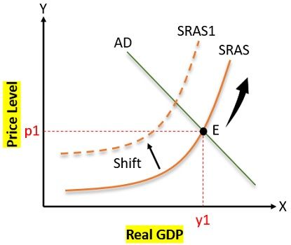
In the above graph,
SRAS is an abbreviation for Short Run Aggregate Supply,
AD represents Aggregate Demand,
E stands for Equilibrium.

In the short term, the prices of goods and services rise slowly. Here, the changes are unpredictable. Moreover, some firms cannot adjust their prices in response to sudden changes in demand.

Long Run Aggregate Supply Curve

It comprises only variable factors. It does not depend on the price level that’s why the total supply curve is a vertical line.

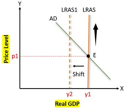
In the above graph, LRAS is an abbreviation for Long Run Aggregate Supply.

The producers get an advantage of the duration and enough planning time. Thus, the change, in the long run, can be predicted and forecasted.

Basically, these changes are triggered by the following factors:

• Technology
• Industrial Changes
• Labour
• Capital Stock

Formula

We can calculate the Aggregate Supply by summation of Total Consumption and Savings. Expressed in the form of formula as:

AS = C + S

Where,
AS stands for Aggregate Supply,
C is Consumption,
S is Savings

We can calculate the Total Income for the entire economy using the same formula. While calculating the total output, firms consider all the factor inputs used in production. Also, we calculate the National Income based on these factor inputs.

Thus, we can conclude that Aggregate Supply is equal to National Income.

Components

Based on the above formula, there are two significant components of total output given below:

1. Consumption
2. Savings

Income is primarily used for Consumption, and the balance left is saved.

It is a part of Income which is not consumed and is referred to as Savings.

Besides these, we need to study those components which cause a shift in the Total Output Curve.

• Technology: Any change in the current technology increases the efficiency of plants. Thus, the producers can increase their output level.
• Exchange Rate: It plays a vital role in determining products cost. As the changes in the exchange rates lead to fluctuation in the product’s price.
• Facility Layout: Any changes in the size of the facility can increase or decrease the production volume.
• Labour Cost: Labour is an essential factor of production. The increase in the wages given to them hypes the product cost, thereby making it expensive.
• Inputs: The fluctuations in the Inputs price impact the product price changes. Further, it increases or decreases the supply levels.

Example

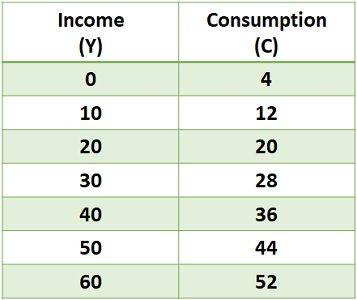
We will learn to find and plot AS using the below table:

Solution

To find and plot AS, you need to prepare an aggregate supply schedule. In this schedule, firstly, we calculate savings by deducting consumption from income.

After that, we will calculate AS by adding consumption and saving.

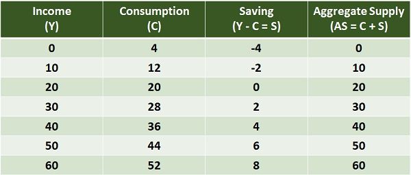
Here, one must note that in this schedule, the Y and AS are the same. Hence, it is proved that Y is equal to AS.

We will plot this schedule on the graph by taking Income on the X-axis and Aggregate Supply on the Y-axis.

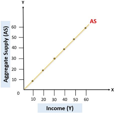
It is evident that the AS curve is making a 45-degree angle, as discussed in the above sections.

Bottom Line

All in all, it indicates the monetary value of the products or output supplies in the economy. In addition, it is the actual amount of goods that the producers wish to offer. We analyse it for a specific duration at a different price level.

Besides, in the economy, the firm’s behaviour is influenced by the producer’s actions. Thus, studying aggregate demand and supply is a must for the smooth functioning of the economy.