Definition: An isoquant curve is that convex shaped curve which is formed by joining the points depicting the different blends of the two production factors, providing constant output. Here, the term ‘isoquant’ can be cracked into ‘iso’ which implies equal and ‘quant’ that stands for quantity. The word altogether means the same volume or constant output at all points.
The production indifference curve works based on diminishing marginal rate of technical substitution of the production factors.
Content: Isoquant Curve
Example
Given below is an isoquant schedule for the various labour and capital combinations which can be made when the output is 1000 Kgs at each time:
| Combination | Labour Units | Capital Units | Output (Kg) | Marginal Rate of Technical Substitution (ΔL/ΔK) |
|---|---|---|---|---|
| A | 1 | 12 | 1000 | _ |
| B | 2 | 8 | 1000 | 1:4 |
| C | 3 | 5 | 1000 | 1:3 |
| D | 4 | 3 | 1000 | 1:2 |
| E | 5 | 2 | 1000 | 1:1 |
Marginal Rate of Technical Substitution (MRTS)
Marginal Rate of Technical Substitution is the proportion at which the one production factor partially replaces the other, to produce consistent output.
MRTS is computed as below:![]()
Where,
L1 is the labour employed in the first combination, and L2 is the labour engaged in the second combination; and
K1 is the capital employed in the first combination and K2 is the capital employed in the second combination.
MRTS keeps on falling at each combination. Thus, the isoquant curve also slopes downwards, as shown below: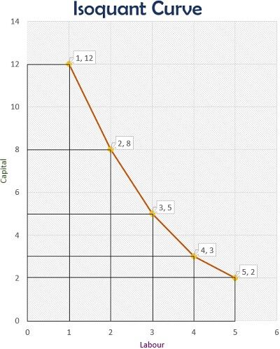
Isoquant Map
An isoquant map is very similar to an indifference map. It can be formed while producing a higher quantity of products from the various possible combinations of the two factors. It facilitates multiple levels of output.
In the given figure we can assume that 1000 units of a product are produced in IQ1, 2000 units in IQ2 and 3000 units in IQ3: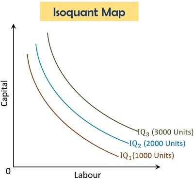
Assumptions for Isoquant Curve
Isoquant curve provides an understanding of how the change in one factor of production affects the other when the output remains constant.
To form an isoquant curve, we have to presume the following:
- Optimum Combinations: All the possible combinations of the production factors are efficient, yielding the same output and quality.
- Two Factors of Production: There are only two factors involved in the production function, as we can say that ‘Q=f(L, K)’.
- Steady Production Technique: The production method or technology remains static throughout the process.
- Technical Substitution Possible: The factors of production should be such that it is possible to substitute one with the other, like labour and capital.
- Divisible Factors of Production: The production factors should be quantifiable or divisible into lesser units or smaller proportion.
Properties of Isoquant Curve
Do you remember the indifference curve we have previously discussed?
The indifference curve is in terms of consumption while the isoquant curve is in the context of the production.
Following are the properties of an isoquant curve:
Convex to the Origin: Since one production factor increases while the other decreases, a convex shaped curve to the origin point, is formed. Another reason for it is the diminishing MRTS.
Right Isoquant Indicates Higher Output than Left Isoquant: When there are more than one isoquant curves on a graph, the upper curve will always indicate a higher output. As in the above isoquant map, IQ2 and IQ3 produce more than IQ1.
Two or More Isoquants May or May Not Be Parallel: As the MRTS of each isoquant curve may vary from one another, two or more isoquant curves don’t need to be parallel to each other.
Negative Slope: To increase the number of units for one factor, the producer has to decrease the units of the other production factor. This principle leads to negative sloping of the isoquant curve.
Two or More Isoquants Never Intersect: As we already know that on an isoquant map, all the isoquant curves depict a different level of output, we can say that they cannot have any combination of factors in common. Thus, the two curves can never intersect one another.
No Isoquant Cuts on Any of the Axis: In industrial application, no commodity can be produced using only one production factor. Therefore, an isoquant curve cannot touch the x or y-axis at any point.
Oval Shaped Curve: An isoquant curve forms a semi-oval shape since it passes through the combinations which show the competent use of the production factors.
Types of Isoquants
While going through the isoquant curves, we come across the numerous possibilities which may or may not be practically applicable.
Let us now discuss some of the most common types of isoquants along with their images below:
Linear Isoquant
It is quite an unrealistic approach where one factor completely substitutes the other in the production process. When the isoquant curve intersects x-axis, capital is entirely replaced by the labour.
Also, when the curve crosses the y-axis, the production is done through capital itself, without employing any labour.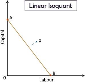
Smooth Convex Isoquant
The isoquant in which there can be only two possible combinations say A and B, except this the two factors of production are incapable of substituting each other.
Thus a smooth convex curve is formed from A to B.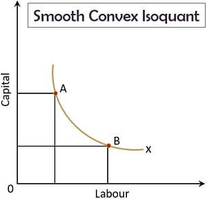
Leontief or Right Angled Isoquant
When the two factors of production cannot be replaced by one another, a right-angled isoquant curve is formed.
Here, the optimum level of production takes place at the edge of the curve or ‘L’. Also, the output remains the same throughout.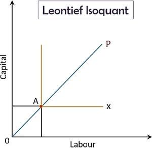
Kinked Isoquant
In such an isoquant curve, the factors of production can substitute each other to a limited extent.
Also, there are a limited number of production processes to support this substitution.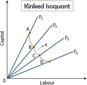
Conclusion
Isoquant curve can be an indicator of efficiently utilizing the two input factors for improving productivity. The production factors involve cost and determining an isoquant curve helps to reduce the unnecessary expenses on these inputs.
vatika says
very nice
Dipankar says
Getting this economics article about isoquant helpfull
शंकर says
best explained. Very satisfied
Aman Asefa says
can you help me economics assignment?